What you'll learn in this lesson
In this tutorial, you'll learn how to:
- Set up your data in Excel so it is in a format that you can use for a pivot table.
- Create a pivot table with that data
- Change the pivot table report to reflect different views on the same data.
The data we'll work with in this example is an Excel table that has two months of daily sales data for a team of four sales people, broken down by product. The first few rows are shown below:
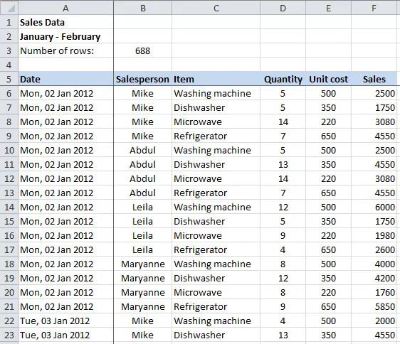
In fact, this spreadsheet extends down for 688 rows of sales data, for all of January and February. So while you might look at the data in the table above and think "I could summarise that quickly by hand or with a few clever formulas", the likelihood is that it would all get too much - and would certainly take too long to do by hand. That's where pivot tables are by far the best solution - you'll be able to convert this data in under a minute, and be able to get different summaries with a few clicks of the mouse.
Getting started with Pivot Tables - make sure your data is ready
There are some important rules you need to follow if you want to create a pivot table from your data:
- You need to have a your data organised in columns with headings. These headings will be used when you create the pivot table, and things will get very confusing without headings.
- Make sure there are no empty columns or rows in your data. Excel is good at sensing the start and end of a data table by looking for empty rows and columns at which point it stops.
- A quick tip to check if your data is formatted in one contiguous range (a fancy term way of saying "one block of data") is to click a single cell in the table then press SHIFT+* (or CTRL+SHIFT+8). This automatically selects the whole table. You'll then see if you have any problems with the layout of your table.
- Note that empty cells are OK. What isn't OK is a whole row or a whole column of empty cells.
- Consistent data in all cells.
- If you have a date column, make sure all the values in that column are dates (or blank).
- If you have a quantity column, make sure all the values are numbers (or blank) and not words.
At this point, if everything is looking OK, you're ready to move on to the next step.
Create a blank Pivot Table
To start your pivot table, follow these steps:
- Click on a cell in the data table. Any cell will do, provided your data meets the rules outlined above. In fact, at this point it's all or nothing - select the whole table or just one cell in the table. Don't select a few cells, because Excel may think you are trying to create a pivot table from just those cells.
- Click on the Insert menu and click the PivotTable button:

- The following dialog box will appear:
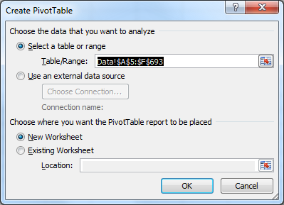
- Note that the Table/Range value will automatically reflect the data in your table (you can click in the field to change the Table/Range value if Excel guessed wrong). Alternatively, you can choose an external data source such as a database (we'll cover that another day!)
- Also notice that you can choose where the new PivotTable should go. By default, Excel will suggest a New Worksheet, which I think is the best choice unless you already know you want it on an existing worksheet.
- Be warned that if your data changes a lot, or you find yourself changing the Pivot Table layout a lot, then refreshing the data in your Pivot Table can result in the Pivot Table changing shape and covering a larger area. If you have data or formulas in that area, they'll disappear. Therefore, putting a Pivot Table on the same page as data or other information can cause you real headaches later on, and thats' why New Worksheet is the recommended option.
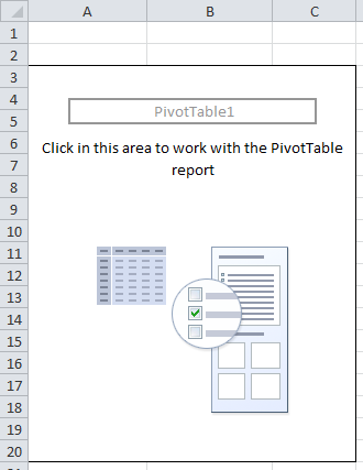
Once you've completed your selections, click OK. Assuming you chose the New Worksheet option, Excel will create a new worksheet in the current workbook, and place the blank PivotTable in the worksheet for you. You are now ready to design your Pivot Table.
Designing your PivotTable layout.
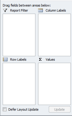
- When you switch to the worksheet with your new Pivot Table, you'll notice three separate elements of the Pivot Table on the screen, starting with the PivotTable report itself:
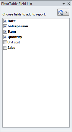
- Then you'll see the Pivot Table Field List and under that the field layout area. Note that it should show the column headings from your data table.
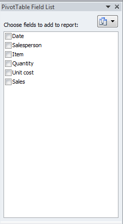
- To create the layout, you need to first select the fields you want in your table, and then place them in the correct location.
- You can check the boxes for the fields you want to include, and Excel will guess which area each field should be placed in. However, the Pivot Table is recalculated each time you check one of the boxes which can slow you down, especially if Excel places a field in the wrong place.
- Therefore, I recommend you drag and drop each field to the area you want it to be.
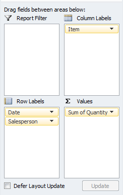
- As an example, here are the Field List and the Field Layout area above with the fields in place to show a report with:
- Each day down the left, with each sales person listed separately for each day
- Items shown across the top.
- The total quantity of items sold for each cell in the Pivot Table.
- Here is how to layout this report:
- The report that this generates looks like this:
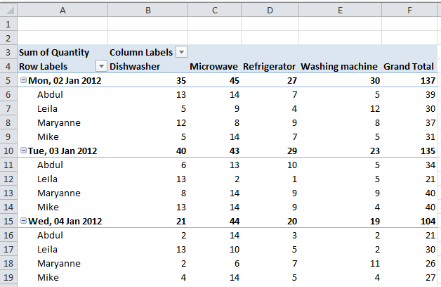
- Notice how the Pivot Table has automatically created a list of the sales people for each day covered in the source data.
Hopefully this lesson has got you started with PivotTables. If you're looking for more, this book by Bill Jelen is well worth a look.
--
We are also on Face Book, Click on Like to jois us
FB Page: https://www.facebook.com/pages/Hyderabad-Masti/335077553211328
FB Group: https://www.facebook.com/groups/hydmasti/
https://groups.google.com/d/msg/hyd-masti/GO9LYiFoudM/TKqvCCq2EbMJ
---
You received this message because you are subscribed to the Google Groups "Hyderabad Masti" group.
To unsubscribe from this group and stop receiving emails from it, send an email to hyd-masti+unsubscribe@googlegroups.com.
For more options, visit https://groups.google.com/groups/opt_out.
No comments:
Post a Comment