[HM:258267] 10 Super Neat Ways to Clean Data in Excel Spreadsheets

​

​

Data forms the backbone of any analysis that you do in Excel. And when it comes to data, there are tons of things that can go wrong – be it the structure, placement, formatting, extra spaces, and so on..

In this blog post, I will show you 10 simple ways to clean data in Excel.

#1 Get Rid of Extra Spaces

Extra spaces are painfully difficult to spot. While you may somehow spot the extra spaces between words or numbers, trailing spaces are not even visible. Here is a neat way to get rid of these extra spaces – Use TRIM Function.

Syntax: TRIM(text)

TRIM function takes the cell reference (or text) as the input. It removes leading and trailing spaces as well as the additional spaces between words (except single spaces).

#2 Select and Treat All Blank Cells

Blank cells can create havoc if not treated beforehand. I often face issues with blank cells in a data set that is used to create reports/dashboards.

You may want to fill all blank cells with '0' or 'Not Available', or may simply want to highlight it. If there is a huge data set, doing this manually could take hours. Thankfully, there is a way you can select all the blank cells at once.

1. Select the entire data set
2. Press F5 (this opens the Go To dialogue box)
3. Click on Special… button (at the bottom left). This opens the Go To Special dialogue box
   
4. Select Blank and Click OK
   

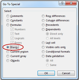
This selects all the blank cells in your data set. If you want to enter 0 or Not Available in all these cells, just type it and press Control + Enter (remember if you press only enter, the value is inserted only in the active cell).

#3 Convert Numbers Stored as Text into Numbers

Sometimes when you import data from text files or external databases, numbers get stored as text. Also, some people are in the habit of using apostrophe (') before a number to make it text. This could create serious issues if you are using these cells in calculations. Here is a fool proof way to converts these numbers stored as text back into numbers.

1. In any blank cell, type 1
2. Select the cell where you typed 1, and press Control + C
3. Select the cell/range which you want to convert to numbers
4. Select Paste –> Paste Special (Key Board Shortcut – Alt + E + S)
5. In the Paste Special Dialogue box, select Multiply (in operations category)
   
6. Click OK. This converts all the numbers in text format back to numbers.

There is a lot more you can do with paste special operations options. Here are various other ways to multiply in Excel using Paste Special.

#4 – Remove Duplicates

There can be 2 things you can do with duplicate data – Highlight It or Delete It.

• Highlight Duplicate Data:
  • Select the data and Go to Home –> Conditional Formatting –> Highlight Cells Rules –> Duplicate Values.
  • Specify the formatting and all the duplicate values get highlighted.
    
• Delete Duplicates in Data: 
  • Select the data and Go to Data –> Remove Duplicates.
  • If your data has headers, ensure that the checkbox at the top right is checked.
  • Select the Column(s) from which you want to remove duplicates and click OK.
    

This removes duplicate values from the list. If you want the original list intact, copy-paste the data at some other location and then do this.

Related: The Ultimate Guide to Find and Remove Duplicates in Excel.

#5 Highlight Errors

There are 2 ways you can highlight Errors in Data in Excel:

Using Conditional Formatting

1. Select the entire data set
2. Go to Home –> Conditional Formatting –> New Rule
3. In New Formatting Rule Dialogue Box select 'Format Only Cells that Contain'
4. In the Rule Description, select Errors from the drop down
5. Set the format and click OK. This highlights any error value in the selected data-set
   

Using Go To Special

1. Select the entire data set
2. Press F5 (this opens the Go To Dialogue box)
3. Click on Special Button at the bottom left
4. Select Formulas and uncheck all options except Errors
   

This selects all the cells that have an error in it. Now you can manually highlight these, delete it, or type anything into it.

#6 Change Text to Lower/Upper/Proper Case

When you inherit a workbook or import data from text files, often the names or titles are not consistent. Sometimes all the text could be in lower/upper case or it could be a mix of both. You can easily make it all consistent by using these three functions:

LOWER() –  Converts all text into Lower Case.
UPPER() – Converts all text into Upper Case.
PROPER() – Converts all Text into Proper Case.

#7 Parse Data Using Text to Column

When you get data from a database or import it from a text file, it may happen that all the text is cramped in one cell. You can parse this text into multiple cells by using Text to Column functionality in Excel.

1. Select the data/text you want to parse
2. Go To Data –> Text to Column (This opens the Text to Columns Wizard)
   • Step 1: Select the data type (select Delimited if you data in not equally spaced, and is separated by characters such as comma, hyphen, dot..). Click Next
     
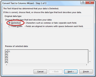
   • Step 2: Select Delimiter (the character that separates your data). You can select pre-defined delimiter or anything else using the Other option
     
   • Step 3: Select the data format. Also select the destination cell. If destination cell is not selected, the current cell is overwritten
     

Related: Extract username from email id using text to column.

#8 Spell Check

Nothing lowers the credibility of your work than a spelling mistake. Use keyboard shortcut F7 to run a spell check for you data set.

Here is a detailed tutorial on how to use Spell check in Excel.

#9 Delete all Formatting

In my job, I used multiple databases to get the data in excel. Every database had it's own data formatting. When you have all the data in place, here is how you can delete all the formatting at one go:

1. Select the data set
2. Go to Home –> Clear –> Clear Formats
   

Similarly, you can also clear only the comments, hyperlinks, or content.

 #10 Use Find and Replace to Clean Data in Excel

Find and replace is indispensable when it comes to data cleansing. For example, you can select and remove all zeros, change references in formulas, find and change formatting, and so on..

http://trumpexcel.com/2014/08/clean-data-in-excel/

--
--
We are also on Face Book, Click on Like to jois us
FB Page: https://www.facebook.com/pages/Hyderabad-Masti/335077553211328
FB Group: https://www.facebook.com/groups/hydmasti/
 
https://groups.google.com/d/msg/hyd-masti/GO9LYiFoudM/TKqvCCq2EbMJ

---
You received this message because you are subscribed to the Google Groups "Hyderabad Masti" group.
To unsubscribe from this group and stop receiving emails from it, send an email to hyd-masti+unsubscribe@googlegroups.com.
For more options, visit https://groups.google.com/d/optout.